In this wave of excitement over Large Language Models (LLMs), one of the most interesting technologies that emerges from them is the idea of embeddings. Most people interact with LLMs (like ChatGPT or Bing Chat) by providing an input and watching it build astonishing output:

Write me a 2-line poem about a carrot whose dream of becoming a banker has gone unfulfilled.

He wanted to be a banker, but he was just a carrot.
He tried to crunch the numbers, but he could not bear it.

https://bing.com/chat

Under the covers, LLMs take the prompted text and turn it into an embedding which is a vector of numbers representing the meaning and context of the tokens processed by the model. In essence (in my non-ML expert view), the embedding represents the model’s conceptual understanding of the input. It then uses this to generate its output.

[-0.003150753309585745, -0.012415633924448732, 0.0095910591273366, -0.0013784545438399322, -0.025483625805167297, …

The first few numbers of an example embedding.

But skipping to the generated output misses the fascinating possibilities embeddings represent. Quantifying a concept numerically opens many opportunities for manipulating semantic understanding. This numerical representation enables scenarios like semantic document search, classification, and translation. Over the last year, many companies have sprung up to take advantage of this potential.

To learn more, I built a program to explore the power of embedding, understand how they work, and learn how to manipulate them. This program takes a document (PDF) as an input and uses embeddings to semantically group and name its key concepts.

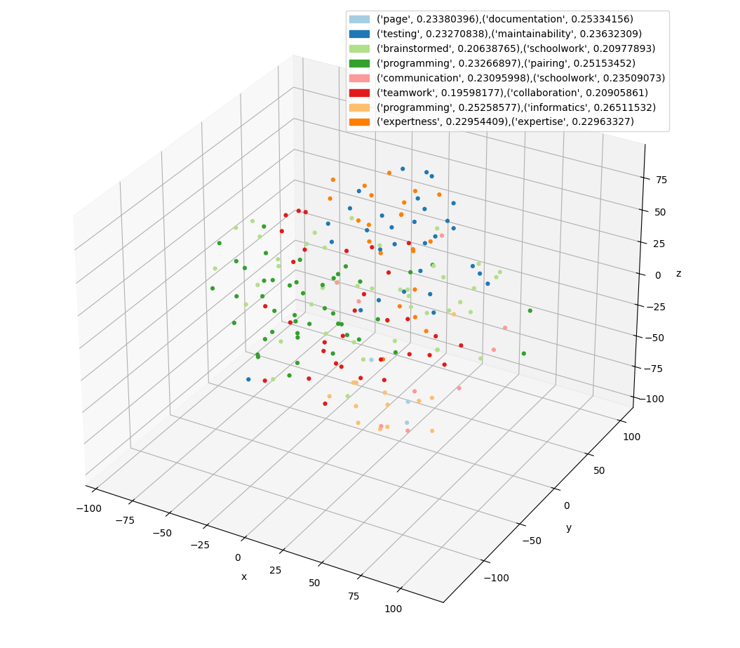
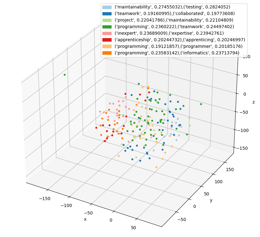
For example, one of the outputs the program can generate is a 3D scatter plot where each dot represents the embedding of an individual section of the document. The color represents a grouping of all similar passages, and the legend shows the words that summarize that grouping.

This post will cover the steps followed to build this program:

Each step will share the key pieces of code needed and show examples for executing that functionality in the program so you can explore and iterate as well. The goal of this post is to demonstrate the power of embeddings and help you get started quickly, leveraging it for your own applications.

If you speak code and not text, jump right to the GitHub repo.

Technology decisions

The program is built in Python which has a rich ecosystem for exploring LLMs and machine learning concepts. It leverages the awesome LangChain library which provides an abstraction for all things language models to enable experimentation.

It also uses OpenAI‘s text-embedding-ada-002 model as the backing LLM. OpenAI API integration is not free, so I purchased $5 worth of tokens. In all my experimentation and testing, I have only used up 10 cents of that amount since the datasets are small. If any cost is prohibitive, LangChain supports different LLMs (both online and local).

Document Splitting and Chunking

The first step is taking an input PDF document and splitting it into smaller chunks. This is required since most LLMs have a character limit. Smaller blocks of text also aid in semantic analysis since larger blocks may contain many concepts and clustering will be less accurate.

LangChain supports many options and configurations for splitting a document. I experimented with three different splitters and with different chunk sizes.

1. RecursiveCharacterTextSplitter – Attempts to chunk a document by using a set of separators.
2. SpacyTextSplitter – Splits text using spaCy’s understanding of English language via its built-in tokenizers.
3. NLTKTextSplitter – Splits text using NLTK’s understanding of English language via its built-in tokenizers.

I split documents many times using each of these text splitters with chunk sizes of 100, 250, 500 and 1000 characters. The chunk size is a suggestion, and it will break the text as close to that as it can. Through this iteration, NLTKTextSplitter showed the best results, but all were reasonable.

This function takes a PDF and chunks it and returns the results:

from langchain.text_splitter import NLTKTextSplitter
from langchain.document_loaders import PyPDFLoader
import os

def parse_pdf(filename):
    path = os.path.join(FILES_FOLDER, filename)
    if not os.path.exists(path):
        raise FileNotFoundError(f'File {path} not found')
 
    chunk_size = 250
    chunk_overlap = 0
    loader = PyPDFLoader(path) 
    nltk_splitter = NLTKTextSplitter(
        chunk_size=chunk_size, chunk_overlap=chunk_overlap)
    texts = loader.load_and_split(text_splitter=nltk_splitter)
    print(f'Loaded {len(texts)} texts')
    return texts

When using NLTK there is a onetime step to download its sentence tokenizing module by running the follow code:

import nltk
nltk.download('punkt')

This functionality is exposed for experimentation in the program through the extract command (referencing the sample pdf included). It prints out the first 100 characters of the first 10 chunks it creates.

./run.sh -m extract -f pair_programming.pdf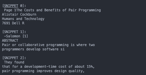

Creating and Querying Embeddings

Generating Embeddings

With bite-sized chunks of text produced, the next task is turning each of these chunks into an embedding. An embedding is a numerical representation of the LLM’s conceptual understanding of the chunk of text. I leveraged LangChain’s OpenAI’s embedding model (OpenAIEmbeddings) and its embeddings caching layer (CacheBackedEmbeddings).

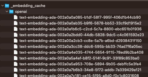
The caching layer minimizes how much it costs (which in hindsight is very small) and improves performance in subsequent runs. It hashes each chunk of text and stores it in a file (or Redis or in memory) per hash with its embeddings.

Using these two classes, this is how to generate embeddings for an array of strings.

from langchain.embeddings import CacheBackedEmbeddings, OpenAIEmbeddings
from langchain.storage import LocalFileStore

# Create a file store to store the cached embeddings
embedding_cache_store = LocalFileStore(EMBEDDING_CACHE_PATH)

# Create an open ai embedding service
underlying_embeddings = OpenAIEmbeddings(
    openai_api_key=os.environ.get('OPENAI_API_KEY'))
    
# Wrap the embedding service in a cache
cached_embedder = CacheBackedEmbeddings.from_bytes_store(
    underlying_embeddings, embedding_cache_store, namespace=underlying_embeddings.model)

# Generate embeddings for the array of texts returned from parse_pdf
doc_embeddings = cached_embedder.embed_documents(texts)

Running it generates the cached embeddings:

With embeddings created and cached, the next step is to load and query them. This enables two key scenarios:

1. Querying embeddings by input text to find closest matches
2. Clustering a list of embeddings

Using a Vector Database

A vector database is the key technology involved in scenario #1. This is a special database that is optimized for storing and querying against vectors of values (like embeddings!). It is built to run in memory or on disk and can scale to very large datasets. LangChain makes it simple to experiment with several vector DBs and I decided to use FAISS. Creating and persisting a FAISS index to disk for the text and embeddings above is just two lines of code:

faiss_index = FAISS.from_texts(texts, cached_embedder)
faiss_index.save_local(VECTOR_STORE_PATH, fileName)

Technically, you don’t need to save the index to disk, since it can be re-built from the cached embeddings, but for large datasets it can save the re-indexing time.

With the index built there is a simple method to provide it a text query and find out which embeddings match most closely:

# Load the index
faiss_index = FAISS.load_local(
    folder_path=VECTOR_STORE_PATH, index_name=fileName, embeddings=cached_embedder)

# Query 3 closest matching chunks from the index
docs_and_scores = faiss_index.similarity_search_with_score(query, 3)
snippet_and_score = [(x[0].page_content[0:100], x[1])
                        for x in docs_and_scores if x[0].page_content]

Storing Embeddings with their chunks

In addition to the vector DB, it is useful to have a persisted list of source text, metadata and embedding. This makes it easy to do further analysis and comparison. There is not a simple way (in my experimenting) to re-construct this from the FAISS index. Instead, store a file to disk that contains all text chunks and their embeddings. To do this, I created a small object called `EmbeddedReference` that contains the embedding, its source text and the page number in the source doc the text came from. I then serialize this to disk.

embedding_objects: list[EmbeddedReference] = []
for i, embedding in enumerate(doc_embeddings):
    embedding_objects.append(EmbeddedReference(
        embedding=embedding, metadata=metadata[i] if metadata is not None else None, content=texts[i]))
with open(paths.get('embeddingStorePath'), 'wb') as f: 
    pickle.dump(embedding_objects, f, pickle.HIGHEST_PROTOCOL)

Then to read this back out and generate a list of the embeddings:

embedding_objects: list[EmbeddedReference] = None
with open(mapPath, 'rb') as f:
    embedding_objects = pickle.load(f)

embeddingsArr = np.array([x.embedding for x in embedding_objects])

Exploring the embedding model

The create command demonstrates taking an input PDF, chunking it, generating embeddings, and storing it to disk as cached embeddings, a vector store and the custom serialized model.

./run.sh -m create -f pair_programming.pdf

After the create command is run once, the query command lets you run queries against the built and persisted model. It takes an input string and returns (by leveraging the vector DB) the first 100 characters of three chunks of text in the document that are semantically closest to the input query.

./run.sh -m query -q "code clarity is a key indicator of success"  -f pair_programming.pdf

# Outputs - first 100 characters of three closest matches
# [
#('[11].”In keeping with the known characteristics of code reviews, we find practitioners citing:• Mi', 0.34571558), 
# ('Coding standards are followed more accurately with the peer pressure to do so• Team members lea', 0.3501709), 
# ('The staff agreed with my points that pair programming: - Should significantly reduce the risk of su', 0.3555439)
#]

Clustering and visualizing embeddings

Generating clusters from embeddings

With the ability to generate, store and query embeddings solved, the next challenge is to demonstrate how the embeddings represent concepts. The key idea is to cluster the embeddings and see what groupings emerged and what they represent. Python has a very rich ecosystem for number analysis and since embeddings are just vectors of numbers all the popular Python libraries like Numpy, Scikit-learn and Pandas can manipulate them. The program leverages the scikit-learn suite for its pre-built clustering algorithms. Clustering is a deep area and many of the modern algorithms can be very complex. Among the different algorithms I experimented with (HDBScan, MiniBatchKMeans, Optics), MiniBatchKMeans showed the best results.

The following code shows how to cluster embeddings and references the embeddingsArr defined in the previous example.

# Runs the clustering algorithm over an array of embeddings (which themselves are long arrays)
clusters = MiniBatchKMeans().fit(embeddingsArr) 

# Get a set of all labels (e.x. 1,2,3,4,5)
labelSet = set([x for x in clusters.labels_ if x != -1])

# Get total number of labels (e.x. 5)
labelCount = len(labelSet)

The output of the clustering algorithm is a set of labels (clusters.labels_) with a label per input embedding. This tells you which group the clustering algorithm assigned to that embedding.

But how do we know if those groupings make sense? The labels are just a number with no innate meaning. This led to the next challenge of visualizing the results of the clustering to understand what (if anything) the grouping of chunks labeled 0, 1 or 2 have in common.

Visualizing clusters

The application generates three visualizations for the clustered embeddings:

1. A histogram of the frequency of the labels
2. A scatter plot of the embeddings in 3-dimensional space with labels mapped to colors
3. A data table for inspecting the chunks and their labels

Histogram

The histogram of label and chunk counts is created using the Matplotlib library in combination with Numpy’s histogram method.

color_palette = sns.color_palette('Paired', labelCount + 1)

# Render histogram of the clusters
labels = np.array(clusters.labels_)
hist, bin_edges = np.histogram(
    labels, bins=range(-1, labelCount + 1))
fig1 = plt.figure()
f1 = fig1.add_subplot()
f1.bar(bin_edges[:-1], hist, width=1, ec="black", color=[
    (0.5, 0.5, 0.5), *color_palette])
plt.xlim(min(bin_edges), max(bin_edges))
f1.set_xlabel('Cluster')
f1.set_ylabel('Count')
f1.grid(True)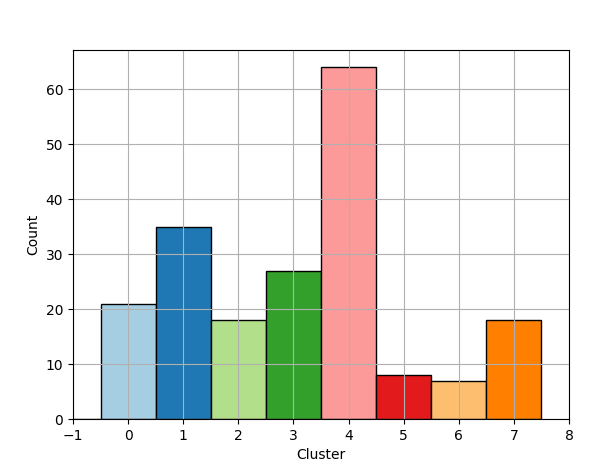

3D Scatter Plot

Generating the scatter plot is more complicated. The problem is that embeddings are 1500 numbers long and to plot in 3D we need to reduce the dimensionality. There are many techniques to do this but the t-SNE (T-distributed Stochastic Neighbor Embedding) library in Scikit-Learn worked well for this case.

t-SNE [1] is a tool to visualize high-dimensional data. It converts similarities between data points to joint probabilities and tries to minimize the Kullback-Leibler divergence between the joint probabilities of the low-dimensional embedding and the high-dimensional data. t-SNE has a cost function that is not convex, i.e., with different initializations we can get different results.

t-SNE takes the 1500-dimension embedding vectors and projects them to 3-dimensionql vectors minimizing the probabilistic difference between the full and reduced data set. With the vector space in 3D, Matplotlib’s scatter chart can plot it. Each clustered label is mapped to a different color. The interesting result is that there are two representations of “similarity”. One is from the clustering algorithm represented by points in the graph with the same color. The other is by points in the graph visually close to each other due to the projection by t-SNE. Based on the analysis, the clustering algorithm’s labelling is more accurate, likely because it has more information at its disposal (all 1500 dimensions).

# Project the embeddings to 3 dimensions
projection = TSNE(n_components=3).fit_transform(embeddingsArr)

 
# Scatter plot by first projecting the n-dimensional embeddings into 3D
# then by using the cluster from HBSCAN to color the points
color_palette = sns.color_palette('Paired', labelCount + 1)
cluster_colors = [color_palette[x] if x >= 0
                  else (0.5, 0.5, 0.5)
                  for x in clusters.labels_] 
                  
fig2 = plt.figure(figsize=(10, 10))
ax = fig2.add_subplot(projection='3d')
ax.scatter(*projection.T, linewidth=0,
           c=cluster_colors, alpha=1)
ax.set_xlabel('x')
ax.set_ylabel('y')
ax.set_zlabel('z')
 
plt.show()

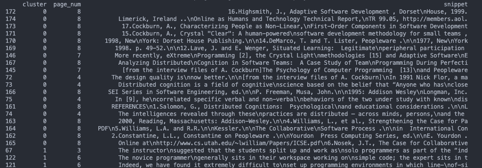
Data Table

The last visualization is a data table to show the results in a readable manner. The Pandas library’s `DataFrame` is used to generate a table with the cluster’s label and first 100 characters of the embeddings source text.

df = pd.DataFrame({
    "cluster":  clusters.labels_,  
    "page_num": [embedding_object.metadata['page'] for embedding_object in embedding_objects],
    "snippet": [embedding_object.content[0:100] for embedding_object in embedding_objects], 
})

df = df.sort_values(by=['cluster'])
print(df.to_string())

This prints a table which I spent time analyzing and trying to figure out which concepts it was grouping by.

Semantically Labelling Each Cluster

Grouping the chunks of text semantically together and manually looking for conceptual similarities is interesting, but we can further leverage embeddings to name the concepts the clusters represent automatically. The approach I took is to generate embeddings for each word in the dictionary. Then by leveraging the vector DB we can find the words closest to each cluster. To represent the cluster as a single point in embedding space we find its centroid (the geometric average of all the embeddings). This builds on the idea that the position in the 1500-dimensional embedding space has semantic meaning, and the average of the points represent a common meaning of them all. This is an intriguing thought and worthy of further exploration to understand change of conceptual meaning by traversing the embedding space.

Generating word embeddings

I use the SCOWL database of English words (which I learned about on a previous project) as the dictionary. It provides word lists categorized by commonality (list 10 being the most common words through list 90 being the least). Combining word lists 10 through 70 yielded the best results.

This list when concatenated all together is 111,814 words long! After analyzing it, I noticed there is a very large amount of the same word with different endings (like biologist and biologists). To minimize these, I used the lemmatization processing class in NLTK called WordNetLemmatizer to post-process the word list. This results in a new word list of length 88,314. This process does not yield perfect results but helps lessen the potential dupe word meanings.

The following code shows how to lemmatize a list of words.

import os 
from nltk.stem import WordNetLemmatizer

with open(WORDS_FILE, 'r') as file:
    words = file.readlines()

wnl = WordNetLemmatizer()

stemmed_words = set([wnl.lemmatize(word.strip())
                    for word in words if len(word) > 0])
sorted_words = sorted(stemmed_words)

With the list of words saved, we can iterate over that list and generate embeddings for each one and persist them to disk in the same way as the chunks of the document.

word_embeddings = cached_embedder.embed_documents(sorted_words)

Exploring word embeddings

In the application the command create_dict generates the embeddings for all 80,000 words. This takes a long time to run so be patient with it.

./run.sh -m create_dict

Once that has finished successfully, the query_dict command takes an input string and finds top 3 closest words (and includes their Euclidean distance from the query text) in the embedding space.

./run.sh -m query_dict -q "If every instinct you have is wrong, then the opposite would have to be right.

# Outputs
# [('contrapositive', 0.3559821), 
#  ('wrongness', 0.35792178), 
#  ('instinct', 0.35800213)]

Labeling the clusters

With the word embeddings built, we generate the describing words for each cluster by calculating the centroid (the average of all the embeddings in the cluster) and finding the words closest to the centroid.

By converting the embeddings into a Numpy array we can use its mean function to calculate the array of averages. For each cluster calculate this average and pass this vector into the vector DB similarity_search_with_score_by_vector method to find the words that best describe that cluster.

# Enumerate each cluster label
for cluster in labelSet:
  print(f'Finding centroid for Cluster {cluster}')
  
  # Calculate the centroid for the cluster
  cluster_embeddings = np.array([x for i, x in enumerate(
     embeddingsArr) if clusters.labels_[i] == cluster])
  mean = cluster_embeddings.mean(axis=0)
  
  print(f'Centroid for cluster {cluster} is {mean}')
  
  # Use the centroid to find words to summarize the cluster
  word_matches = words_index.similarity_search_with_score_by_vector(
      mean, 3)
  word_and_scores = [(x[0].page_content[0:SNIPPET_LENGTH], x[1])
                     for x in word_matches if x[0].page_content]
  print(f'Words for cluster {cluster} are {word_and_scores}')
  
  # Use tuple of top two matching words to categorize the groups
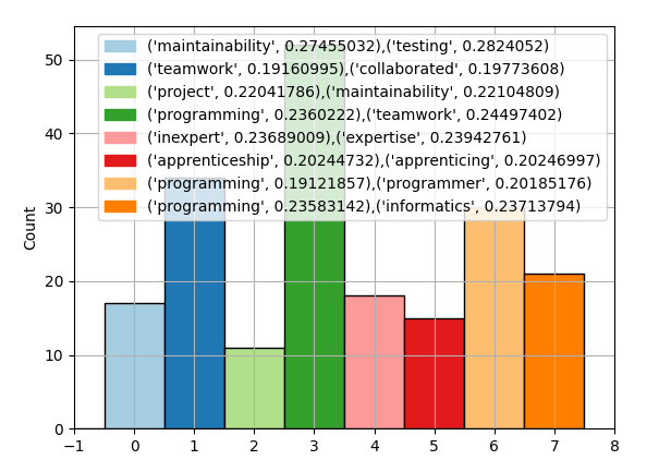
  clusterCategory[cluster] = f'{word_and_scores[0]},{word_and_scores[1]}'

Initially, I labelled each cluster with the topmost closest word match, but this led to several distinct clusters labeled with the same word: programming. If the article is primarily about programming, it makes sense that core topic in each chunk of text will match closely with that word. Including the second closest word adds much more clarity on the intent of that passage. For example, in one test two chunks of text that were labeled with “programming” changed to “programming, teamwork” and “programming, testing” respectively. Both clusters of passages are still about programming, but one set focuses more on teamwork while the other on testing.

With the word labels created, we can update the graphs from earlier to add a legend naming each cluster. For example, the following shows adding the legend to the histogram:

color_palette = sns.color_palette('Paired', labelCount + 1)

# Render histogram of the clusters
labels = np.array(clusters.labels_)
hist, bin_edges = np.histogram(
    labels, bins=range(-1, labelCount + 1))
fig1 = plt.figure()
f1 = fig1.add_subplot()
f1.bar(bin_edges[:-1], hist, width=1, ec="black", color=[
    (0.5, 0.5, 0.5), *color_palette])
plt.xlim(min(bin_edges), max(bin_edges))
f1.set_xlabel('Cluster')
f1.set_ylabel('Count')
f1.grid(True)

# Addition to add a legend
handles = []
for cluster in set(labels):
    if cluster >= 0:
        handles.append(
            mpatches.Patch(color=color_palette[cluster], label=clusterCategory[cluster]))
    else:
        handles.append(
            mpatches.Patch(color=(0.5, 0.5, 0.5), label='None'))
f1.legend(handles=handles)

To generate the final charts showing the 3D scatter plot and the histogram with the categorized cluster labels, run the analyze command.

./run.sh -m analyze -f pair_programming.pdf 

Which outputs:

Conclusion

It is deeply intriguing thinking about ideas existing in a N-dimensional space and using distance calculations to find interrelations between concepts. This program only scratches the surface on the possibilities in this space. The tools and libraries that have grown around LLM’s (like LangChain) make exploration in this space easy and understandable. I am eager to see and read more and hopefully experiment further on the power of embeddings.

The finished application is available on GitHub, check it out and let me know what you think.